Update: See the cooling as an animated gif.
Did you know it is cooling on the west coast of North America from 1983 to 2011? Before I show you how I found that out and what I found, I will tell you a story.
About a month ago I was reading the Victoria Times Colonist and read an article titled Warmer weather in B.C. threatens waterfront, forests. The key sentence to me was “An analysis of 62 years of Environment Canada weather data by the University of Victoria’s Pacific Climate Impacts Consortium has found that B.C.’s temperature has been warming by about 0.25 degrees Celsius per decade” which came from this report .
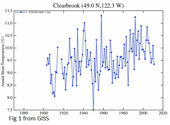
My first thought was “No Way”. I live in BC. It hasn’t been warming recently. But how was I to prove otherwise? I sent an email to Francis Zwiers who is the Director and I sent him a couple of screen shots from GISS from a few nearby climate stations showing that it has been warmer , and recently it hasn’t been warming. I sent a screenshot of Clearbrook (and a few others) which is right on the border with BC in Washington State. Fig 1 Clearbrook from GISS.

The key number in the quote was 62 years, which means they were using 1950 as a starting year. Clearbrook exhibits one of the common signatures of west coast climate stations – 1950 was amazingly cold. You can see that temperatures dropped 3.5C from 1940 to 1950.1950 on the west coast is kind of like a micro Little Ice Age. Sure it warmed after 1950 because every year was warmer than 1950.
After a few emails back and forth I asked for his data. Guess what he said? “It’s publically available from Environment Canada.” Sound familiar? That kind of ticked me off. To be fair, after a couple more emails he offered to send me the data and also pointed me at an Environment Canada website where I could scrape it myself or I could wait for the public access portal they were planning.
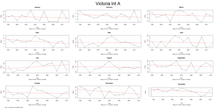
By then I had decided it was time to learn R. I wrote an R script to scrape the EC site for data and then I came across a tip that would allow me to segment a plot into 12 subplots and thought why not show each month. I picked Victoria Int A from 1998 to 2011. I chose to take the lm (linear model) value from [R] and multiply it by 10 to show the trend in C per decade.
Fig 2 – Victoria Int A 1998 to 2011

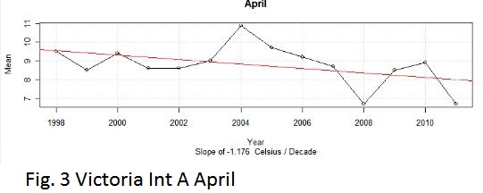
Even though it was an airport some months were cooling. Fig. 3 Victoria April 1998 to 2011

Then the BEST data came out with a new release. I decided to compare BEST with Environment Canada and found some interesting things out. But that’s a different story. I decided to rewrite my [R] script and analyze the Quality Controlled release, and I came up with another idea of “mapping” the stations by color (red for warming and blue for cooling) against latitude and longitude.
The code to do Victoria (or any other station) is not complex. Assuming you have the BEST data loaded as BESTdata and the column names are Year, Tm, Month and Station_ID here is a snippet of code to graph Victoria.
months <- c(“January”,”February”,”March”,”April”,”May”,”June”,”July”,”August”,”September”,”October”,”November”,”December”)
dev.new(width=1200,height=800)
split.screen( figs = c( 4, 3 ) )
par( oma = c( 0, 0, 3, 1 ) )
sid<- 7998
dfOneStation <- subset(BESTdata,Station_ID == sid & Year >= 1990,select=c(Year,Tm,Month))
decslope.all <- 0
decslope.count <- 0
for (i in 1:12) {
screen(i)
dfOneStation.m <- subset(dfOneStation,Month == i )
r = lm(dfOneStation.m$Tm~dfOneStation.m$Year)
Decadal_slope <- round(coef(r)[2],digits=4) * 10
decslope.all <- decslope.all + Decadal_slope
decslope.count <- decslope.count + 1
mTitle = paste(months[i],Decadal_slope,”Celsius/Decade”)
if (Decadal_slope > 0) {
colmain = “red”
} else { colmain = “blue”}
plot(dfOneStation.m$Year,dfOneStation.m$Tm,main=mTitle,type=”o”,xlab=”Year”, ylab=”Temperature”,col.main=colmain)
abline(r,col=colmain)
}
ds <- decslope.all/decslope.count
if (decslope.all > 0) {
colmain = “red”
} else { colmain = “blue”}
mtext(paste(sid,” “,round(ds,digits=4),” Celsius/Decade”,sep = “”,collapse = NULL), outer = TRUE, cex=2,line=1 ,col=colmain)
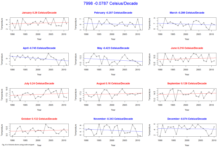
Fig. 4 is Victoria done using code snippet

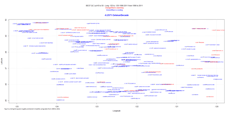
Fig. 5 is a “map” Fig. 5 is a 5×5 grid square centered around Seattle using data from 1990 to 2011 (only stations with data in 1990 and data in 2011) It is really cooling by -.2571 Celsius per decade.

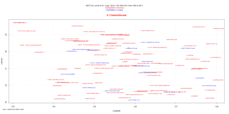
And, just to be fair, Fig. 6 is the same grid square 1945 to 2011. Notice that a few stations are still cooling and the warming trend is only .1C per decade.


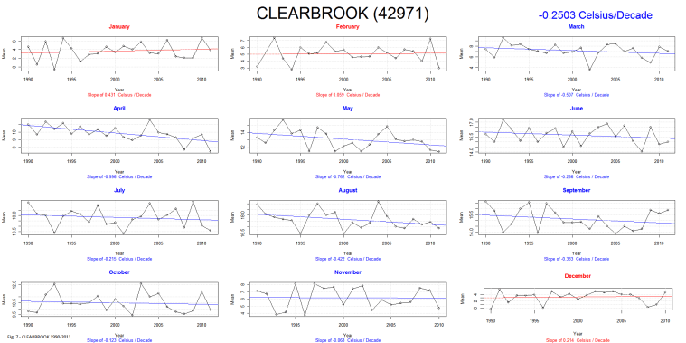
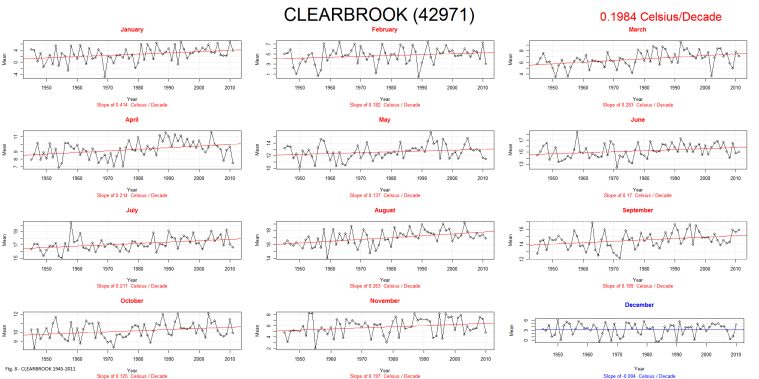
Fig. 7 is Clearbrook for 1990 to 2011 and Fig. 8 is Clearbrook for 1945 to 2011.
Notice that on both graphs there is still one or more months that are contrary to the overall trend. That is quite common. Of course sometimes the trends are quite miniscule one way or the other. And other times they are huge.
After running my script for a few regions I am just amazed at the difference between stations. Fig. 9 is Crete Nebraska, warming at a miniscule .031C/Decade since 1910! And yet July, August, September and October (not shown) are cooling and have never been as warm as the 1930s:

I could bounce all over the world with fascinating examples.
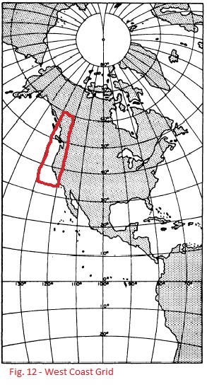
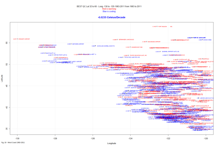
But, is the west coast warming? In this case, by West Coast, I mean a box Latitude 32 to Latitude 60 and Longitude -130 to -120. It is slightly cooling from 1983 to 2011. There appears to have been a climate shift well before the 1998 one seen in the global indexes like CRU. Fig. 10 – West Coast 1983-2011

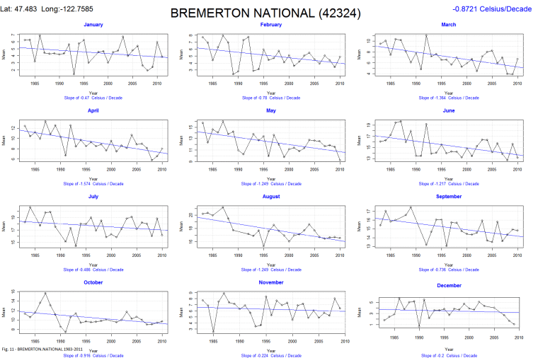
One of the stations with the biggest cooling trend is Bremerton National. It is cooling at a rate of -.87 Celsius/decade. And it is an airport! Fig. 11 – BREMERTON.NATIONAL 1983-2011

The grid I call the West Coast is shown here in Fig. 12
